


6 Lesser-Recognized Scikit-Be taught Options That Will Save You Time
For many individuals finding out information science, Scikit-Learn is usually the primary machine studying library they encounter. It’s as a result of Scikit-Be taught provides numerous APIs which are helpful for mannequin growth whereas nonetheless being straightforward for newbies to make use of.
As useful as they could be, many options from Scikit-Be taught are hardly ever explored and have untapped potential. This text will discover six lesser-known options that may prevent time.
1. Validation Curve
The primary operate we are going to discover is the validation curve operate from Scikit-Be taught. From the title, you possibly can guess that it performs some sort of validation, nevertheless it’s not simply easy validation that’s performs. The operate explores machine studying mannequin efficiency over numerous values of particular hyperparameters.
Utilizing the cross-validation technique, the validation curve operate evaluates coaching and take a look at efficiency over the vary of hyperparameter values. The method ends in two units of scores that we will examine visually.
Let’s check out the operate with pattern information and visualize the outcomes. First, let’s load pattern information and arrange the hyperparameter vary we wish to discover. On this case, we are going to discover how the SVC mannequin’s accuracy efficiency over numerous gamma hyperparameters.
|
1 2 3 4 5 6 7 8 9 10 11 12 13 14 15 16 17 18 |
import numpy as np import matplotlib.pyplot as plt from sklearn.model_selection import validation_curve from sklearn.svm import SVC from sklearn.datasets import load_iris
information = load_iris() X, y = information.information, information.goal
param_range = np.logspace(–3, 3, 5)
train_scores, test_scores = validation_curve( SVC(), X, y, param_name=“gamma”, param_range=param_range, cv=5, scoring=“accuracy” ) |
When you execute the code above, you’ll get two scores: train_scores & test_scores.
These are each assigned arrays of scores like beneath.
|
(array([[0.925 , 0.925 , 0.93333333, 0.925 , 0.9 ], [0.975 , 0.94166667, 0.975 , 0.96666667, 0.95833333], [0.975 , 0.98333333, 0.99166667, 0.99166667, 0.99166667], [1. , 1. , 1. , 1. , 1. ], [1. , 1. , 1. , 1. , 1. ]]), array([[0.86666667, 0.96666667, 0.83333333, 0.96666667, 0.93333333], [0.93333333, 0.96666667, 0.93333333, 0.93333333, 1. ], [0.96666667, 1. , 0.9 , 0.96666667, 1. ], [0.86666667, 0.73333333, 0.7 , 0.8 , 0.9 ], [0.46666667, 0.4 , 0.33333333, 0.4 , 0.4 ]])) |
We will visualize the validation curve utilizing code much like the next.
|
plt.determine(figsize=(8, 6)) plt.plot(param_range, train_mean, label=“Coaching rating”, colour=“blue”, marker=“o”) plt.plot(param_range, test_mean, label=“Cross-validation rating”, colour=“inexperienced”, marker=“s”) plt.xscale(“log”) plt.xlabel(“Gamma”) plt.ylabel(“Accuracy”) plt.title(“Validation Curve for SVC (gamma parameter)”) plt.legend(loc=“greatest”) plt.present() |
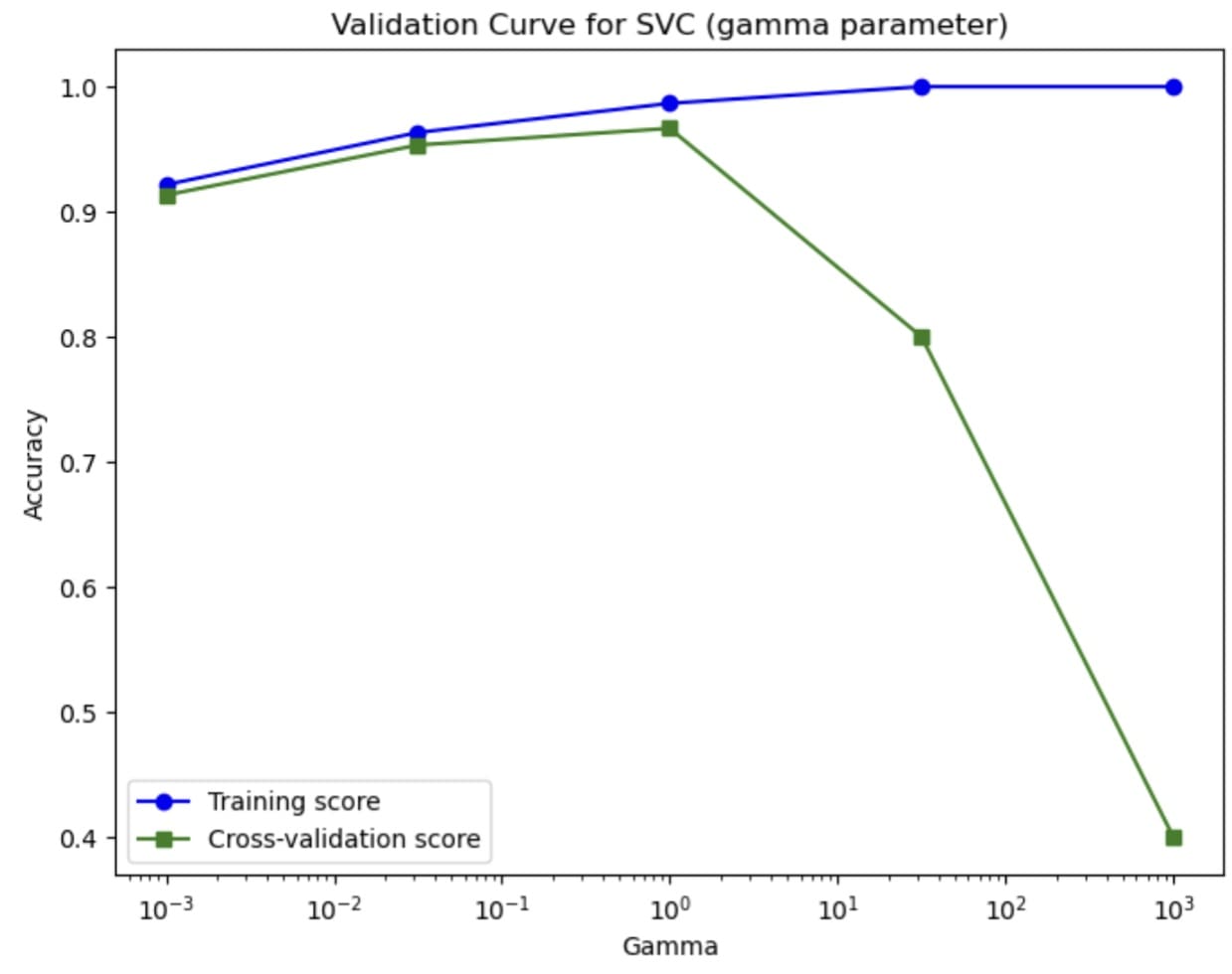
The curve teaches us how the hyperparameters have an effect on the mannequin’s efficiency. Utilizing the validation curve, we will discover the optimum worth for the hyperparameter and estimate it higher than counting on the easy train-test break up.
Strive utilizing a validation curve in your mannequin growth course of to information you in growing the very best mannequin potential and keep away from points akin to overfitting.
2. Mannequin Calibration
After we develop a machine studying classifier mannequin, we have to keep in mind that it’s not sufficient merely to offer right classification prediction; the chances related to the prediction should even be dependable. The method to make sure that the chances are dependable is known as calibration.
The calibration course of adjusts the mannequin’s likelihood estimation. The method pushes the likelihood to mirror the true chance of the prediction so it’s not overconfident or underconfident. The uncalibrated mannequin may predict an occasion with a 90% likelihood likelihood, whereas the precise success fee is way decrease, which suggests the mannequin was overconfident. That’s why we have to calibrate the mannequin.
By calibrating the mannequin, we may enhance the belief in mannequin prediction and inform the person of the particular estimation of the particular danger from the mannequin.
Let’s strive the calibration course of with Scikit-Be taught. The library provides a diagnostic operate (calibration_curve) and a mannequin calibration class (CalibratedClassifierCV).
We’ll use breast most cancers information and the logistic regression mannequin as the idea. Then, we are going to examine the unique mannequin with the calibrated mannequin for the likelihood.
|
1 2 3 4 5 6 7 8 9 10 11 12 13 14 15 16 17 18 19 20 21 22 23 24 25 26 27 28 29 30 |
import numpy as np import matplotlib.pyplot as plt from sklearn.datasets import load_breast_cancer from sklearn.linear_model import LogisticRegression from sklearn.calibration import calibration_curve, CalibratedClassifierCV from sklearn.model_selection import train_test_split
information = load_breast_cancer() X, y = information.information, information.goal
X_train, X_test, y_train, y_test = train_test_split(X, y, random_state=42) lr = LogisticRegression().match(X_train, y_train)
prob_pos_lr = lr.predict_proba(X_test)[:, 1] fraction_lr, mean_pred_lr = calibration_curve(y_test, prob_pos_lr, n_bins=10)
calibrated_clf = CalibratedClassifierCV(lr, cv=‘prefit’, technique=‘isotonic’) calibrated_clf.match(X_train, y_train) prob_pos_calibrated = calibrated_clf.predict_proba(X_test)[:, 1] fraction_cal, mean_pred_cal = calibration_curve(y_test, prob_pos_calibrated, n_bins=10)
plt.determine(figsize=(8, 6)) plt.plot(mean_pred_lr, fraction_lr, marker=‘o’, label=‘Authentic LR’) plt.plot(mean_pred_cal, fraction_cal, marker=‘s’, label=‘Calibrated LR (Isotonic)’) plt.plot([0, 1], [0, 1], linestyle=‘–‘, label=‘Excellent Calibration’) plt.xlabel(“Imply predicted likelihood”) plt.ylabel(“Fraction of positives”) plt.title(“Calibration Curve Comparability”) plt.legend(loc=“higher left”) plt.present() |

We will see that the calibrated logistic regression is nearer to the mannequin with excellent calibration than the unique. Which means that the calibrated mannequin can higher estimate the precise danger, though it’s nonetheless not superb.
Strive utilizing the calibration technique to enhance the mannequin prediction functionality.
3. Permutation Significance
Every time we work with a machine studying mannequin, we use the info options to offer the prediction consequence. Nevertheless, not each characteristic contributes to the prediction in the identical method.
The permutation_importance() technique is for measuring the characteristic contribution to mannequin performances by randomly permuting (altering) characteristic values and evaluating the mannequin efficiency after the permutation. If the mannequin efficiency degrades, the characteristic impacts the mannequin; conversely, if the mannequin efficiency is unchanged, it means that the characteristic may not be that helpful for the precise mannequin efficiency.
The method is easy and intuitive, making it useful in decoding any mannequin’s inner decision-making. It’s useful for fashions with no inherent characteristic significance technique embedded inside.
Let’s check out the mannequin with a Python code instance. We’ll use pattern information and fashions much like our earlier instance.
|
import numpy as np import matplotlib.pyplot as plt from sklearn.datasets import load_iris from sklearn.linear_model import LogisticRegression from sklearn.inspection import permutation_importance from sklearn.model_selection import train_test_split
information = load_iris() X, y = information.information, information.goal
X_train, X_test, y_train, y_test = train_test_split(X, y, random_state=42)
mannequin = LogisticRegression() mannequin.match(X_train, y_train)
consequence = permutation_importance(mannequin, X_test, y_test, n_repeats=10, random_state=42, scoring=‘accuracy’) |
With the code above, we now have the mannequin and permutation significance consequence, the place we are going to analyze the characteristic’s impression on the mannequin. Let’s have a look at the typical and normal deviation outcomes for permutation significance.
|
feature_names = information.feature_names importances = consequence.importances_mean std = consequence.importances_std
for i, title in enumerate(feature_names): print(f“{title}: Imply significance = {importances[i]:.4f} (+/- {std[i]:.4f})”) |
The result’s as follows.
|
sepal size (cm): Imply significance = 0.0132 (+/– 0.0177) sepal width (cm): Imply significance = 0.0000 (+/– 0.0000) petal size (cm): Imply significance = 0.6000 (+/– 0.0805) petal width (cm): Imply significance = 0.1553 (+/– 0.0362) |
We will additionally visualize the consequence above to know the mannequin efficiency higher.
|
plt.barh(feature_names, importances, xerr=std) plt.xlabel(“Lower in accuracy”) plt.title(“Permutation Significance”) plt.present() |
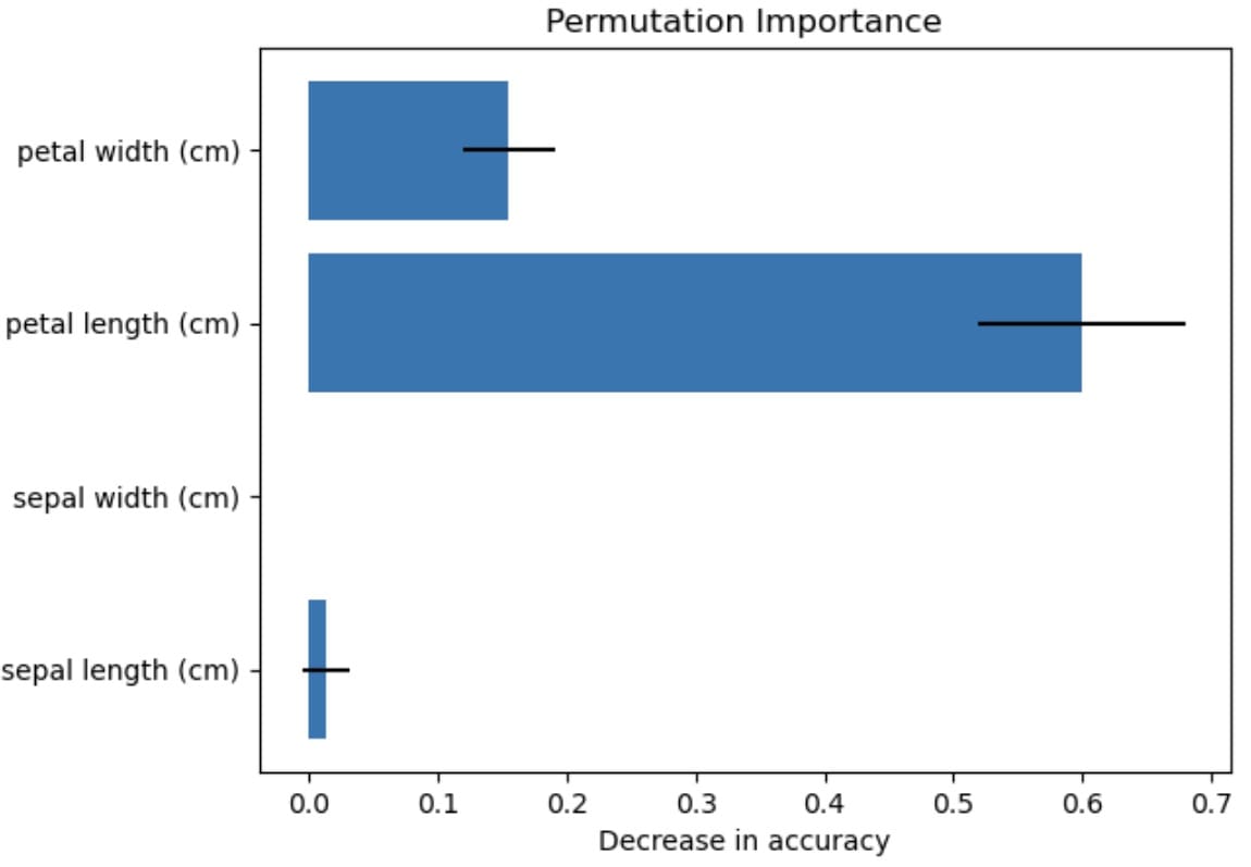
The visualization reveals that the petal size most impacts the characteristic efficiency, whereas the sepal width has no impact. There may be all the time uncertainty, which is represented by the usual deviation, however we will conclude with the permutation significance method that petal size has probably the most impression.
That’s a easy characteristic significance method that you should use in your subsequent undertaking.
4. Characteristic Hasher
Engaged on options for information science modeling, I usually discovered that high-dimensional options have been too reminiscence intensive, which impacted the appliance’s general efficiency. There are lots of methods to enhance efficiency, akin to dimensionality discount or characteristic choice. The hashing technique is one other technique that may be hardly ever used however may very well be useful.
Hashing is changing information right into a sparse numeric matrix with a set measurement. Making use of a hash operate to every characteristic can map the represented characteristic right into a sparse matrix. We’ll use a hash operate by way of FeatureHasher to compute the matrix column similar to a reputation.
Let’s strive it out with the Python code.
|
import pandas as pd import seaborn as sns from sklearn.feature_extraction import FeatureHasher
titanic = sns.load_dataset(“titanic”)
titanic_sample = titanic[[‘sex’, ’embarked’, ‘class’]].dropna()
data_dicts = titanic_sample.to_dict(orient=‘information’) hasher = FeatureHasher(n_features=10, input_type=‘dict’)
hashed_features = hasher.rework(data_dicts)
hashed_array = hashed_features.toarray() print(“nHashed characteristic matrix (dense format):n”, hashed_array) |
You will note the output appears to be like just like the one beneath.
|
Hashed characteristic matrix (dense format): [[ 1. 0. 0. ... 0. –1. 0.] [–1. 0. 0. ... 0. 0. 0.] [ 1. 0. 0. ... 0. 0. 0.] ... [ 1. 0. 0. ... 0. 0. 0.] [–1. 0. 0. ... 0. –1. 0.] [ 1. 0. 0. ... 0. –1. 0.]] |
The dataset has been represented right into a sparse matrix with 10 completely different options. You possibly can specify the variety of hash options it’s essential to stability the reminiscence utilization and knowledge loss.
5. Strong Scaler
Actual-world information is never clear, and most of the time riddled with outliers. Whereas an outlier just isn’t intrinsically dangerous and may give info that contributes to the precise perception, there are occasions when it would skew our mannequin outcomes.
There are lots of methods for scaling our outliers, however typically they’ll introduce bias. That’s why strong scaling is vital to assist preprocess our information. Strong scaling transforms the info by eradicating the median and scaling them in response to the IQR as a substitute of utilizing imply and normal deviation.
The robust scaler is correct, with only some outliers at excessive positions. By making use of it, the dataset is secure and never influenced a lot by the outliers, which makes it helpful for any machine studying mannequin growth.
Right here is an instance of utilizing the strong scaler. Let’s use the Iris information instance and introduce an outlier within the dataset.
|
import numpy as np import pandas as pd from sklearn.datasets import load_iris from sklearn.preprocessing import robust_scale import matplotlib.pyplot as plt
iris = load_iris() X = iris.information
outlier = np.array([[10, 10, 10, 10]]) X_out = np.vstack([X, outlier])
X_scaled = robust_scale(X_out) |
The above code simply scales the info with our launched outlier. Strive utilizing your self in case you are having a tough time with outliers.
6. Characteristic Union
Feature union is a Scikit-Be taught characteristic that mixes a number of characteristic transformations throughout the pipeline. As an alternative of remodeling the identical options sequentially, characteristic union inputs the info into a number of transformers concurrently to offer all of the remodeled options.
It’s a useful characteristic the place completely different transformers are required to seize numerous elements of information and must be current within the dataset. One transformer may used for the PCA method, whereas the others use strong scaling.
Let’s strive it out with the next code beneath. For instance, we will create transformers for each PCA and polynomial options transformers.
|
1 2 3 4 5 6 7 8 9 10 11 12 13 14 15 16 17 18 19 |
import numpy as np from sklearn.datasets import load_iris from sklearn.decomposition import PCA from sklearn.preprocessing import PolynomialFeatures from sklearn.pipeline import FeatureUnion
information = load_iris() X, y = information.information, information.goal
pca = PCA(n_components=2)
poly = PolynomialFeatures(diploma=2, include_bias=False)
union = FeatureUnion(transformer_list=[ (‘pca’, pca), (‘poly’, poly) ])
X_transformed = union.fit_transform(X) |
The instance results of the remodeled options is proven within the output beneath.
|
[–2.68412563 0.31939725 5.1 3.5 1.4 0.2 26.01 17.85 7.14 1.02 12.25 4.9 0.7 1.96 0.28 0.04 ] |
The consequence comprises the PCA and polynomial options we now have beforehand remodeled.
Strive experimenting with a number of transformations to see in the event that they fit your evaluation.
Conclusion
Scikit-Be taught is a library that many information scientists use to develop fashions simply from their information. It’s straightforward to make use of and offers many options which are helpful for our mannequin work, but lots of these options appear underutilized although they may prevent time.
On this article, we now have explored six of those underutilized options, from validation curves to characteristic hashing to a sturdy scaler that isn’t extremely influenced by outliers. Hopefully you discovered one thing new and of worth herein, and I hope this has helped!
Source link