


Diagnosing and Fixing Overfitting in Machine Studying with Python
Picture by Writer | Ideogram
Introduction
Overfitting is likely one of the most (if not probably the most!) widespread issues encountered when constructing machine studying (ML) fashions. In essence, it happens when the mannequin excessively learns from the intricacies (and even noise) discovered within the coaching knowledge as a substitute of capturing the underlying sample in a means that enables for higher generalization to future unseen knowledge. Diagnosing whether or not your ML mannequin suffers from this drawback is essential to successfully addressing it and guaranteeing good generalization to new knowledge as soon as deployed to manufacturing.
This text, offered in a tutorial type, illustrates tips on how to diagnose and repair overfitting in Python.
Setting Up
We’d like knowledge to coach the mannequin earlier than diagnosing overfitting in an ML mannequin. Let’s begin by importing the required packages and creating an artificial dataset susceptible to overfitting earlier than coaching a regression mannequin upon it.
Loading packages:
|
import numpy as np import matplotlib.pyplot as plt from sklearn.preprocessing import PolynomialFeatures from sklearn.linear_model import LinearRegression from sklearn.pipeline import make_pipeline from sklearn.model_selection import train_test_split from sklearn.metrics import mean_squared_error |
Dataset creation (largely following a sinusoidal sample with some added noise):
|
def generate_data(n_samples=20, noise=0.2): np.random.seed(42) X = np.linspace(–3, 3, n_samples).reshape(–1, 1) y = np.sin(X) + noise * np.random.randn(n_samples, 1) return X, y
X, y = generate_data() X_train, X_test, y_train, y_test = train_test_split(X, y, test_size=0.3, random_state=42) |
Diagnosing Overfitting
There are two widespread approaches to diagnosing overfitting:
- One is by visualizing the mannequin’s predictions or outputs as a operate of inputs in comparison with the precise knowledge. That is doable utilizing plots, particularly for lower-dimensional knowledge, to see if the mannequin is overfitting the coaching knowledge somewhat than capturing the underlying sample in a extra generalizable method.
- For fashions of upper complexity which might be more durable to visualise, one other method is to look at the distinction between the accuracy (or error) within the coaching set and the testing or validation set. A big hole, the place coaching efficiency is considerably higher than check efficiency, is a powerful indicator of overfitting.
Since we can be coaching a really low-complexity polynomial regression mannequin to suit the low-dimensional, randomly generated dataset we created earlier, we’ll now outline a operate that trains a polynomial regression mannequin and visualizes it alongside coaching and check knowledge, as a way for diagnosing overfitting.
|
1 2 3 4 5 6 7 8 9 10 11 12 13 14 15 16 17 18 19 20 |
def train_and_view_model(diploma): mannequin = make_pipeline(PolynomialFeatures(diploma), LinearRegression()) mannequin.match(X_train, y_train)
X_plot = np.linspace(–3, 3, 100).reshape(–1, 1) y_pred = mannequin.predict(X_plot)
plt.scatter(X_train, y_train, coloration=‘blue’, label=‘Prepare knowledge’) plt.scatter(X_test, y_test, coloration=‘purple’, label=‘Check knowledge’) plt.plot(X_plot, y_pred, coloration=‘inexperienced’, label=f‘Poly Diploma {diploma}’) plt.legend() plt.title(f‘Polynomial Regression (Diploma {diploma})’) plt.present()
train_error = mean_squared_error(y_train, mannequin.predict(X_train)) test_error = mean_squared_error(y_test, mannequin.predict(X_test)) print(f‘Diploma {diploma}: Prepare MSE = {train_error:.4f}, Check MSE = {test_error:.4f}’) return train_error, test_error
X_train, X_test, y_train, y_test = train_test_split(X, y, test_size=0.3, random_state=42) |
Let’s name this operate to coach and visualize a polynomial regressor with diploma equal to 10. Basically, the upper the diploma, the extra intricate the polynomial curve can grow to be, therefore the extra tightly it may possibly match the coaching knowledge. Due to this fact, a really excessive polynomial diploma could enhance the chance of a mannequin that overfits the info, and in addition extra unpredictable patterns may be exhibited by the mannequin (curve), as we’ll see shortly.
|
overfit_degree = 10 train_and_view_model(overfit_degree) |
That is the ensuing mannequin and knowledge visualization:
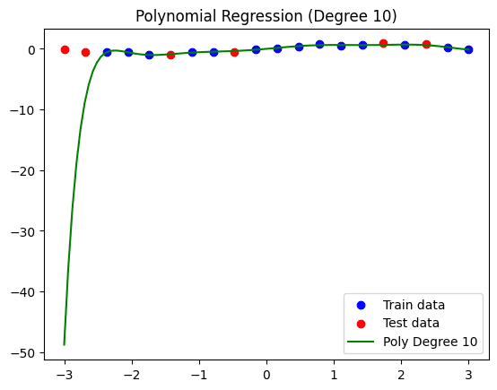
Polynomial regression mannequin (levels = 10).
Notice that the customized operate we outlined earlier than additionally prints the error made in coaching and check knowledge, thus offering one other overfitting analysis method. On this mannequin, we have now a Imply Squared Error (MSE) of 0.0052 on coaching knowledge, and a a lot increased error of 406.1920 on the check knowledge, largely because of the drastic sample seen on the left-hand aspect of the regression curve.
Fixing Overfitting
To repair overfitting on this instance, we’ll apply a easy but usually efficient technique: simplifying the mannequin. For a polynomial regression mannequin, this entails lowering the diploma of the curve. Let’s attempt for example a level equal to three:
|
reduced_degree = 3 train_and_view_model(reduced_degree) |
Ensuing visualization:
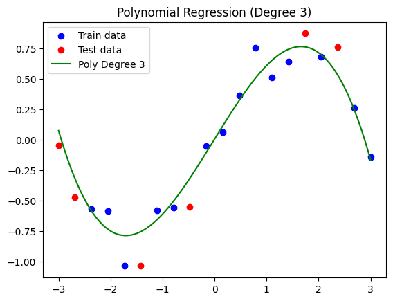
Simplified polynomial regression mannequin (levels = 3).
As we are able to see, whereas this curve doesn’t match the coaching set as a complete as tightly because the earlier mannequin did, we could have overcome the overfitting subject to a point, thus arising with a mannequin that will generalize higher to future distinct knowledge. The ensuing coaching MSE is 0.0139, whereas the check MSE is 0.0394. This time, whereas there may be nonetheless a distinction between the errors, it’s a lot much less drastic: an indication that this mannequin is extra generalizable.
Conclusion
This text unveiled the required sensible steps to find and deal with the overfitting drawback in classical machine studying fashions skilled in Python. Concretely, we illustrated tips on how to spot and repair overfitting in a polynomial regression mannequin by visualizing the mannequin alongside the info, calculating the error made, and simplifying the mannequin to make it extra generalizable.
Source link