


Kernel Strategies in Machine Studying with Python
Picture by Editor | Midjourney
Introduction
Kernel strategies are a robust class of machine studying algorithm that enable us to carry out complicated, non-linear transformations of information with out explicitly computing the remodeled characteristic area. These strategies are notably helpful when coping with high-dimensional knowledge or when the connection between options is non-linear.
Kernel strategies depend on the idea of a kernel perform, which computes the dot product of two vectors in a remodeled characteristic area with out explicitly performing the transformation. This is named the kernel trick. The kernel trick permits us to work in high-dimensional areas effectively, making it potential to resolve complicated issues that may be computationally infeasible in any other case.
Why would we use kernel strategies?
- Non-linearity: Kernel strategies can seize non-linear relationships in knowledge by mapping it to a higher-dimensional area the place linear strategies could be utilized
- Effectivity: Through the use of the kernel trick, we keep away from the computational value of explicitly remodeling the information
- Versatility: Kernel strategies could be utilized to a variety of duties, together with classification, regression, and dimensionality discount
On this tutorial, we’ll discover the basics of kernel strategies, specializing in the next subjects:
- The Kernel Trick: Understanding the mathematical basis of kernel strategies
- Help Vector Machines (SVMs): Utilizing SVMs for classification with kernel features
- Kernel PCA: Dimensionality discount utilizing kernel PCA
- Sensible Examples: Implementing SVMs and Kernel PCA in Python
The Kernel Trick
The kernel trick is a mathematical method that permits us to compute the dot product of two vectors in a high-dimensional area with out explicitly mapping the vectors to that area. That is notably helpful when the transformation to the high-dimensional area is computationally costly and even unimaginable to compute instantly.
A kernel perform ( Okay(x, y) ) computes the dot product of two vectors ( x ) and ( y ) in a remodeled characteristic area:
[
K(x, y) = phi(x) cdot phi(y)
]
Right here, ( phi(x) ) is a mapping from the unique characteristic area to a higher-dimensional area. The kernel perform permits us to compute this dot product instantly within the authentic area.
Frequent kernel features embrace:
- Linear Kernel: ( Okay(x, y) = x cdot y )
- Polynomial Kernel: ( Okay(x, y) = (x cdot y + c)^d )
- Radial Foundation Operate (RBF) Kernel: ( Okay(x, y) = exp(-gamma |x – y|^2) )
The selection of kernel perform relies on the issue at hand. For instance, the RBF kernel is usually used when the information shouldn’t be linearly separable.
Help Vector Machines (SVMs) with Kernel Features
A Help Vector Machine (SVM) is a supervised studying algorithm used for classification and regression duties. The aim of an SVM is to seek out the hyperplane that finest separates the information into totally different lessons. When the information shouldn’t be linearly separable, we will use kernel features to map the information to a higher-dimensional area the place it turns into separable.
Let’s implement a kernel SVM utilizing the scikit-learn library. We’ll use the well-known Iris dataset for classification.
|
1 2 3 4 5 6 7 8 9 10 11 12 13 14 15 16 17 18 19 20 21 22 23 24 25 26 27 28 29 30 31 32 33 34 35 36 37 38 39 40 41 42 43 44 45 |
import numpy as np import matplotlib.pyplot as plt from sklearn import datasets from sklearn.model_selection import train_test_split from sklearn.svm import SVC from sklearn.metrics import accuracy_rating
# Load the Iris dataset iris = datasets.load_iris() X = iris.knowledge[:, :2] # We’ll use solely the primary two options for visualization y = iris.goal
# Break up the information into coaching and testing units X_train, X_test, y_train, y_test = train_test_split(X, y, test_size=0.3, random_state=42)
# Create an SVM classifier with an RBF kernel svm = SVC(kernel=‘rbf’, gamma=0.7, C=1.0)
# Practice the SVM svm.match(X_train, y_train)
# Make predictions y_pred = svm.predict(X_test)
# Consider the mannequin accuracy = accuracy_score(y_test, y_pred) print(f“Accuracy: {accuracy:.2f}”)
# Plot the choice boundary def plot_decision_boundary(X, y, mannequin): h = .02 # Step measurement within the mesh x_min, x_max = X[:, 0].min() – 1, X[:, 0].max() + 1 y_min, y_max = X[:, 1].min() – 1, X[:, 1].max() + 1 xx, yy = np.meshgrid(np.arange(x_min, x_max, h), np.arange(y_min, y_max, h)) Z = mannequin.predict(np.c_[xx.ravel(), yy.ravel()]) Z = Z.reshape(xx.form) plt.contourf(xx, yy, Z, alpha=0.8) plt.scatter(X[:, 0], X[:, 1], c=y, edgecolors=‘ok’, marker=‘o’) plt.xlabel(‘Sepal size’) plt.ylabel(‘Sepal width’) plt.title(‘SVM Determination Boundary with RBF Kernel’) plt.present()
plot_decision_boundary(X_train, y_train, svm) |
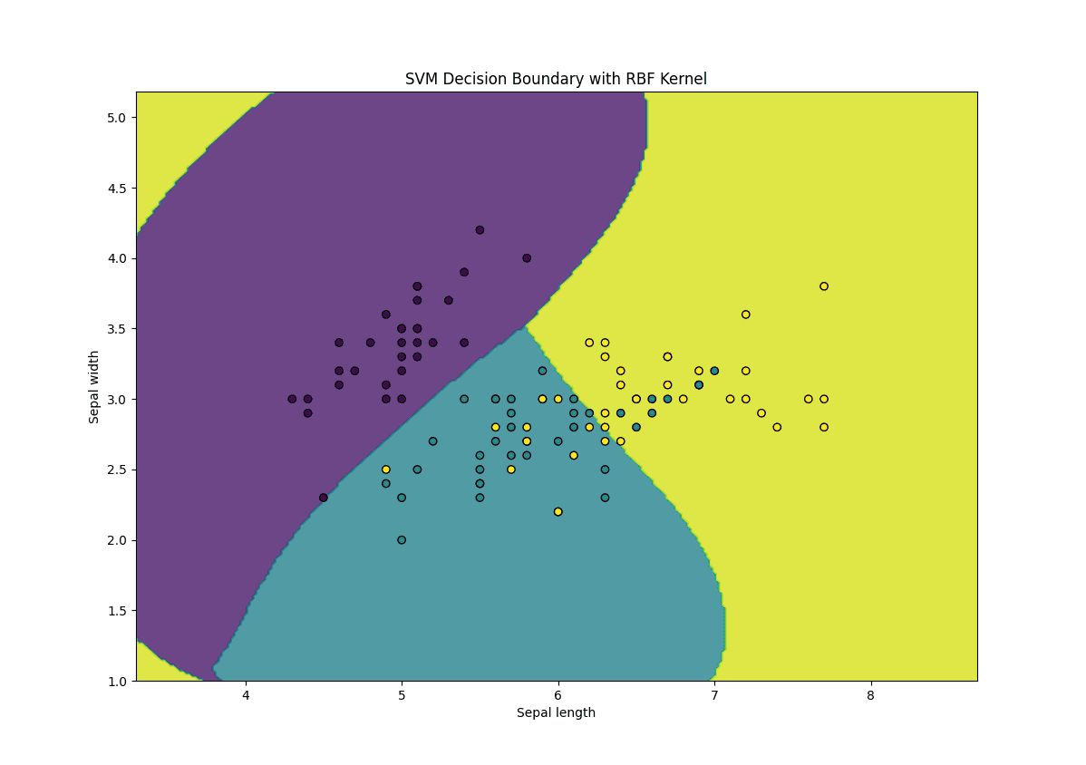
Right here’s what’s happening within the above code:
- Kernel Choice: We use the RBF kernel (kernel=’rbf’) to deal with non-linear knowledge
- Gamma Parameter: The gamma parameter controls the affect of every coaching instance, the place the next gamma worth ends in a extra complicated resolution boundary
- C Parameter: The C parameter controls the trade-off between reaching a low coaching error and a low testing error
Kernel Principal Element Evaluation (Kernel PCA)
Principal Element Evaluation (PCA) is a dimensionality discount method that tasks knowledge onto a lower-dimensional area whereas preserving as a lot variance as potential. Nonetheless, normal PCA is proscribed to linear transformations. Kernel PCA extends PCA through the use of kernel features to carry out non-linear dimensionality discount.
Let’s implement Kernel PCA utilizing scikit-learn and apply it to a non-linear dataset.
|
1 2 3 4 5 6 7 8 9 10 11 12 13 14 15 16 17 18 19 20 21 22 |
from sklearn.decomposition import KernelPCA from sklearn.datasets import make_moons
# Generate a non-linear dataset X, y = make_moons(n_samples=100, noise=0.1, random_state=42)
# Apply Kernel PCA with an RBF kernel kpca = KernelPCA(kernel=‘rbf’, gamma=15, n_components=2) X_kpca = kpca.fit_transform(X)
# Plot the unique knowledge and the remodeled knowledge plt.determine(figsize=(12, 5))
plt.subplot(1, 2, 1) plt.scatter(X[:, 0], X[:, 1], c=y, edgecolors=‘ok’, marker=‘o’) plt.title(‘Unique Information’)
plt.subplot(1, 2, 2) plt.scatter(X_kpca[:, 0], X_kpca[:, 1], c=y, edgecolors=‘ok’, marker=‘o’) plt.title(‘Kernel PCA Remodeled Information’)
plt.present() |
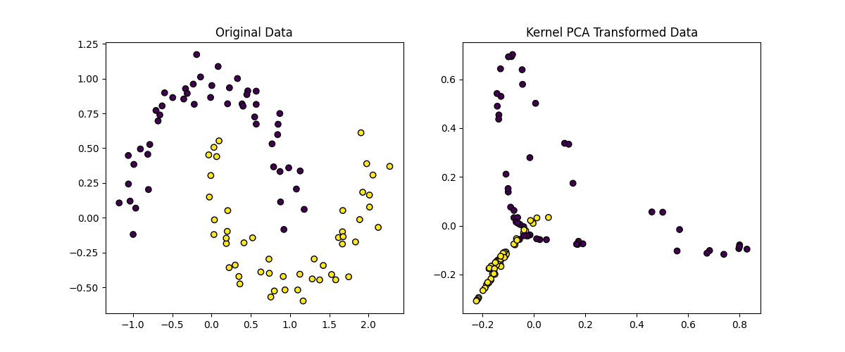
Right here’s an evidence of the code above:
- Kernel Choice: We use the RBF kernel (kernel=’rbf’) to seize non-linear relationships within the knowledge
- Gamma Parameter: The gamma parameter controls the affect of every knowledge level, the place the next gamma worth ends in a extra complicated transformation
- Variety of Elements: We scale back the information to 2 dimensions (n_components=2) for visualization
Implementing the Kernel Trick from Scratch
A fast reminder: the kernel trick permits us to compute the dot product of two vectors in a high-dimensional area with out explicitly mapping the vectors to that area. That is performed utilizing a kernel perform, which instantly computes the dot product within the remodeled area.
Let’s implement the Radial Foundation Operate (RBF) kernel from scratch and use it to compute the kernel matrix for a dataset. The RBF kernel is outlined as:
[
K(x, y) = expleft(-gamma |x – y|^2right)
]
The place:
- ( x ) and ( y ) are knowledge factors
- ( gamma ) is a parameter that controls the affect of every knowledge level, which we’ll consult with as gamma
- ( |x – y|^2 ) is the squared Euclidean distance between ( x ) and ( y )
Step 1: Outline the RBF Kernel Operate
Let’s begin with the RBF kernel perform.
|
import numpy as np
def rbf_kernel(x1, x2, gamma=1.0): “”“ Compute the RBF kernel between two vectors x1 and x2.
Parameters: – x1, x2: Enter vectors. – gamma: Kernel parameter.
Returns: – Kernel worth (scalar). ““” squared_distance = np.sum((x1 – x2) ** 2) return np.exp(–gamma * squared_distance) |
Step 2: Compute the Kernel Matrix
The kernel matrix (or Gram matrix) is a matrix the place every factor ( K_{ij} ) is the kernel worth between the ( i )-th and ( j )-th knowledge factors. Let’s compute the kernel matrix for a dataset.
|
1 2 3 4 5 6 7 8 9 10 11 12 13 14 15 16 17 18 19 20 |
def compute_kernel_matrix(X, kernel_function, gamma=1.0): “”“ Compute the kernel matrix for a dataset X utilizing a given kernel perform.
Parameters: – X: Enter dataset (n_samples, n_features). – kernel_function: Kernel perform to make use of. – gamma: Kernel parameter.
Returns: – Kernel matrix (n_samples, n_samples). ““” n_samples = X.form[0] kernel_matrix = np.zeros((n_samples, n_samples))
for i in vary(n_samples): for j in vary(n_samples): kernel_matrix[i, j] = kernel_function(X[i], X[j], gamma)
return kernel_matrix |
Step 3: Apply the Kernel Trick to a Easy Dataset
Let’s generate a easy 2D dataset and compute its kernel matrix utilizing the RBF kernel.
|
# Generate a easy 2D dataset X = np.array([[1, 2], [2, 3], [3, 4], [4, 5]])
# Compute the kernel matrix utilizing the RBF kernel gamma = 0.1 kernel_matrix = compute_kernel_matrix(X, rbf_kernel, gamma)
print(“Kernel Matrix (RBF Kernel):”) print(kernel_matrix) |
The kernel matrix will look one thing like this:
|
Kernel Matrix (RBF Kernel): [[1. 0.81873075 0.44932896 0.16529889] [0.81873075 1. 0.81873075 0.44932896] [0.44932896 0.81873075 1. 0.81873075] [0.16529889 0.44932896 0.81873075 1. ]] |
Step 4: Use the Kernel Matrix in a Kernelized Algorithm
Now that we’ve the kernel matrix, we will use it in a kernelized algorithm, equivalent to a kernel SVM. Nonetheless, implementing a full kernel SVM from scratch is complicated, so we’ll use the kernel matrix to exhibit the idea.
For instance, in a kernel SVM, the choice perform for a brand new knowledge level ( x ) is computed as:
[
f(x) = sum_{i=1}^n alpha_i y_i K(x, x_i) + b
]
The place:
- ( alpha_i ) are the Lagrange multipliers (discovered throughout coaching).
- ( y_i ) are the labels of the coaching knowledge.
- ( Okay(x, x_i) ) is the kernel worth between ( x ) and the ( i )-th coaching level.
- ( b ) is the bias time period.
Whereas we received’t implement the total SVM right here, the kernel matrix is an important element of kernelized algorithms.
Here’s a abstract of the kernel trick implementation:
- we carried out the RBF kernel perform from scratch
- we computed the kernel matrix for a dataset utilizing the RBF kernel
- the kernel matrix can be utilized in kernelized algorithms like kernel SVMs or kernel PCA
This implementation demonstrates the core thought of the kernel trick: working in a high-dimensional area with out explicitly remodeling the information. You possibly can lengthen this method to implement different kernel features (e.g., polynomial kernel) or use the kernel matrix in customized kernelized algorithms.
Advantages of Kernel Trick vs. Specific Transformation
So, why will we use the kernel trick as an alternative of specific transformation?
Specific Transformation
Suppose we’ve a 2D dataset ( X = [x_1, x_2] ) and we wish to remodel it right into a higher-dimensional area utilizing a polynomial transformation. For simplicity, let’s contemplate a quadratic transformation:
[
phi(x) = [x_1, x_2, x_1^2, x_2^2, x_1 x_2]
]
Right here, ( phi(x) ) maps the unique 2D knowledge right into a 5D area. If we’ve ( n ) knowledge factors, we would wish to compute this transformation for every level, leading to a ( n occasions 5 ) matrix.
|
import numpy as np
# Unique 2D knowledge X = np.array([[1, 2], [2, 3], [3, 4]])
# Specific transformation to 5D area def explicit_transformation(X): x1 = X[:, 0] x2 = X[:, 1] return np.column_stack((x1, x2, x1**2, x2**2, x1 * x2))
# Apply the transformation X_transformed = explicit_transformation(X) print(“Explicitly Remodeled Information:”) print(X_transformed) |
And the output of the above code can be:
|
Explicitly Remodeled Information: [[ 1 2 1 4 2] [ 2 3 4 9 6] [ 3 4 9 16 12]] |
Right here, we explicitly computed the brand new options within the 5D area. This works high quality for small datasets and low-dimensional transformations, but it surely turns into problematic for:
- Excessive-dimensional knowledge: If the unique knowledge has many options, the remodeled area can explode in measurement
- Advanced transformations: Some transformations (e.g., RBF) map knowledge into an infinite-dimensional area, which is unimaginable to compute explicitly.
Let’s now distinction this with the kernel trick.
Kernel Trick
The kernel trick avoids explicitly computing ( phi(x) ) by instantly computing the dot product ( phi(x) cdot phi(y) ) within the remodeled area utilizing a kernel perform ( Okay(x, y) ). For instance, the RBF kernel implicitly maps knowledge into an infinite-dimensional area, however we by no means compute ( phi(x) ) instantly.
|
# Kernel trick: Compute the dot product within the remodeled area with out specific transformation def rbf_kernel(x1, x2, gamma=1.0): squared_distance = np.sum((x1 – x2) ** 2) return np.exp(–gamma * squared_distance)
# Compute the kernel matrix kernel_matrix = compute_kernel_matrix(X, rbf_kernel, gamma=1.0) print(“Kernel Matrix (RBF Kernel):”) print(kernel_matrix) |
And the output:
|
Kernel Matrix (RBF Kernel): [[1.00000000e+00 1.35335283e–01 3.35462628e–04 1.52299797e–08] [1.35335283e–01 1.00000000e+00 1.35335283e–01 3.35462628e–04] [3.35462628e–04 1.35335283e–01 1.00000000e+00 1.35335283e–01] [1.52299797e–08 3.35462628e–04 1.35335283e–01 1.00000000e+00]] |
Right here, we by no means explicitly computed ( phi(x) ). As an alternative, we used the kernel perform to compute the dot product within the remodeled area instantly.
Technique Comparability
Right here’s why specific transformation is problematic:
- Computational Price: Explicitly remodeling knowledge right into a high-dimensional area requires computing and storing the brand new options, which could be computationally costly
- Infinite Dimensions: Some transformations (e.g., RBF) map knowledge into an infinite-dimensional area, which is unimaginable to compute explicitly
- Reminiscence Utilization: Storing the remodeled knowledge can require quite a lot of reminiscence, particularly for giant datasets
Specific transformation TL;DR: Straight computes the remodeled options ( phi(x) ) within the higher-dimensional area. That is possible for easy, low-dimensional transformations however turns into impractical for complicated or high-dimensional transformations.
Conversely, the kernel trick is especially helpful when:
- The remodeled characteristic area could be very high-dimensional or infinite-dimensional
- You wish to keep away from the computational value of explicitly remodeling the information
- You’re working with kernelized algorithms like SVMs, Kernel PCA, or Gaussian Processes
Kernel trick TL;DR: Avoids specific transformation by computing the dot product ( phi(x) cdot phi(y) ) instantly utilizing a kernel perform. That is environment friendly and works even for infinite-dimensional areas. The kernel trick is a intelligent mathematical shortcut that permits us to work in high-dimensional areas with out the computational burden of specific transformation.
Conclusion
Kernel strategies are a robust device in machine studying, enabling us to deal with non-linear knowledge effectively. On this tutorial, we explored the kernel trick, kernel SVMs, and Kernel PCA, and offered sensible Python examples that can assist you get began with these strategies.
By mastering kernel strategies, you’ll be able to sort out a variety of machine studying issues, from classification to dimensionality discount, with better flexibility and effectivity.
Source link