


Mastering Time Collection Forecasting: From ARIMA to LSTM
Picture by Editor | Midjourney
Introduction
Time collection forecasting is a statistical approach used to investigate historic knowledge factors and predict future values primarily based on temporal patterns. This methodology is especially invaluable in domains the place understanding developments, seasonality, and cyclical patterns drives crucial enterprise selections and strategic planning. From predicting inventory market fluctuations to forecasting power demand spikes, correct time collection evaluation helps organizations optimize stock, allocate sources effectively, and mitigate operational dangers. Fashionable approaches mix conventional statistical strategies with machine studying to deal with each linear relationships and complicated nonlinear patterns in temporal knowledge.
On this article, we’ll discover three predominant strategies for forecasting:
- Autoregressive Built-in Transferring Common (ARIMA): A easy and common methodology that makes use of previous values to make predictions
- Exponential Smoothing Time Collection (ETS): This methodology seems at developments and patterns over time to offer higher forecasts
- Lengthy Brief-Time period Reminiscence (LSTM): A extra superior methodology that makes use of deep studying to know advanced knowledge patterns
Preparation
First, we import the required libraries.
|
# Import vital libraries import pandas as pd import numpy as np import matplotlib.pyplot as plt from statsmodels.tsa.arima.mannequin import ARIMA from statsmodels.tsa.stattools import adfuller from statsmodels.tsa.holtwinters import ExponentialSmoothing from prophet import Prophet from sklearn.model_selection import train_test_split from sklearn.preprocessing import MinMaxScaler from keras.fashions import Sequential from keras.layers import LSTM, Dense, Enter |
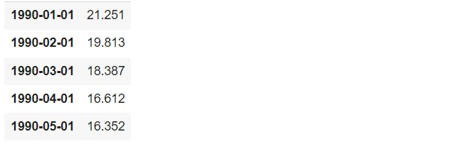
Then, we load the time collection and look at its first few rows.
|
# Load your dataset df = pd.read_csv(‘timeseries.csv’, parse_dates=[‘Date’], index_col=‘Date’) df.head() |
1. Autoregressive Built-in Transferring Common (ARIMA)
ARIMA is a well known methodology used to foretell future values in a time collection. It combines three elements:
- AutoRegressive (AR): The connection between an remark and quite a few lagged observations
- Built-in (I): The differencing of uncooked observations to permit for the time collection to turn into stationary
- Transferring Common (MA): The connection reveals how an remark differs from the anticipated worth in a shifting common mannequin utilizing previous knowledge
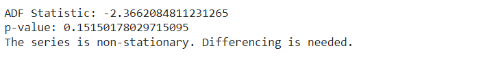
We use the Augmented Dickey-Fuller (ADF) check to examine if our knowledge stays the identical over time. We take a look at the p-value from this check. If the p-value is 0.05 or decrease, it means our knowledge is secure.
|
# ADF Check to examine for stationarity consequence = adfuller(df[‘Price’])
print(‘ADF Statistic:’, consequence[0]) print(‘p-value:’, consequence[1])
if consequence[1] > 0.05: print(“The collection is non-stationary. Differencing is required.”) else: print(“The collection is stationary.”) |
We carry out first-order differencing on the time collection knowledge to make it stationary.
|
# First-order differencing df[‘Differenced’] = df[‘Price’].diff()
# Drop lacking values ensuing from differencing df.dropna(inplace=True)
# Show the primary few rows of the differenced knowledge print(df[[‘Price’, ‘Differenced’]].head()) |

We create and match the ARIMA mannequin to our knowledge. After becoming the mannequin, we forecast the long run values.
|
# Match the ARIMA mannequin mannequin = ARIMA(df[‘Price’], order=(1, 1, 1)) model_fit = mannequin.match()
# Forecasting subsequent steps forecast = model_fit.forecast(steps=10) |
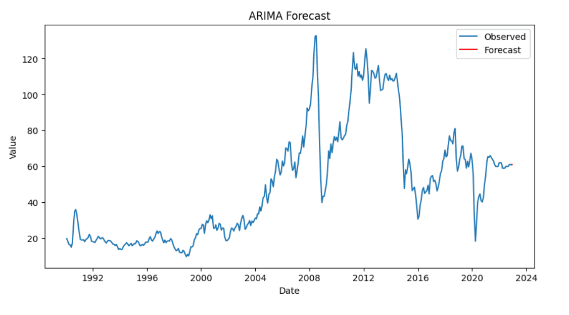
Lastly, we visualize our outcomes to match the precise and predicted values.
|
# Plotting the outcomes plt.determine(figsize=(10, 5)) plt.plot(df[‘Price’], label=‘Noticed’) plt.plot(pd.date_range(df.index[–1], intervals=10, freq=‘D’), forecast, label=‘Forecast’, shade=‘purple’) plt.title(‘ARIMA Forecast’) plt.xlabel(‘Date’) plt.ylabel(‘Worth’) plt.legend() plt.present() |
2. Exponential Smoothing Time Collection (ETS)
Exponential smoothing is a technique used for time collection forecasting. It contains three elements:
- Error (E): Represents the unpredictability or noise within the knowledge
- Pattern (T): Reveals the long-term course of the information
- Seasonality (S): Captures repeating patterns or cycles within the knowledge
We are going to use the Holt-Winters methodology for performing ETS. ETS helps us predict knowledge that has each developments and seasons.
|
# Match the ETS mannequin (Exponential Smoothing) ets_model = ExponentialSmoothing(df[‘Price’], seasonal=‘add’, pattern=‘add’, seasonal_periods=12) ets_fit = ets_model.match() |
We generate forecasts for a specified variety of intervals utilizing the fitted ETS mannequin.
|
# Forecasting the subsequent 12 intervals forecast = ets_fit.forecast(steps=12) |
Then, we plot the noticed knowledge together with the forecasted values to visualise the mannequin’s efficiency.
|
# Plot noticed and forecasted values plt.determine(figsize=(10, 6)) plt.plot(df, label=‘Noticed’) plt.plot(forecast, label=‘Forecast’, shade=‘purple’) plt.title(‘ETS Mannequin Forecast’) plt.xlabel(‘Date’) plt.ylabel(‘Value’) plt.legend() plt.present() |

3. Lengthy Brief-Time period Reminiscence (LSTM)
LSTM is a kind of neural community that appears at knowledge in a sequence. It’s good at remembering necessary particulars for a very long time. This makes it helpful for predicting future values in time collection knowledge as a result of it might discover advanced patterns.
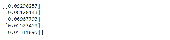
LSTM is delicate to scale of the information. So, we alter the goal variable to ensure all values are between 0 and 1. This course of known as normalization.
|
# Extract the values of the goal column knowledge = df[‘Price’].values knowledge = knowledge.reshape(–1, 1)
# Normalize the information scaler = MinMaxScaler(feature_range=(0, 1)) scaled_data = scaler.fit_transform(knowledge)
# Show the primary few scaled values print(scaled_data[:5]) |
LSTM expects enter within the type of sequences. Right here, we’ll cut up the time collection knowledge into sequences (X) and their corresponding subsequent worth (y).
|
# Create a operate to transform knowledge into sequences for LSTM def create_sequences(knowledge, time_steps=60): X, y = [], [] for i in vary(len(knowledge) – time_steps): X.append(knowledge[i:i+time_steps, 0]) y.append(knowledge[i+time_steps, 0]) return np.array(X), np.array(y)
# Use 60 time steps to foretell the subsequent worth time_steps = 60 X, y = create_sequences(scaled_data, time_steps)
# Reshape X for LSTM enter X = X.reshape(X.form[0], X.form[1], 1) |
We cut up the information into coaching and check units.
|
# Break up the information into coaching and check units (80% prepare, 20% check) train_size = int(len(X) * 0.8) X_train, X_test = X[:train_size], X[train_size:] y_train, y_test = y[:train_size], y[train_size:] |
We are going to now construct the LSTM mannequin utilizing Keras. Then, we’ll compile it utilizing the Adam optimizer and imply squared error loss.
|
1 2 3 4 5 6 7 8 9 10 11 12 13 14 15 16 17 |
from keras.fashions import Sequential from keras.layers import LSTM, Dense, Enter
# Initialize the Sequential mannequin mannequin = Sequential()
# Outline the enter layer mannequin.add(Enter(form=(time_steps, 1)))
# Add the LSTM layer mannequin.add(LSTM(50, return_sequences=False))
# Add a Dense layer for output mannequin.add(Dense(1))
# Compile the mannequin mannequin.compile(optimizer=‘adam’, loss=‘mean_squared_error’) |
We prepare the mannequin utilizing the coaching knowledge. We additionally consider the mannequin’s efficiency on the check knowledge.
|
# Prepare the mannequin on the coaching knowledge historical past = mannequin.match(X_train, y_train, epochs=20, batch_size=32, validation_data=(X_test, y_test)) |
After we prepare the mannequin, we’ll use it to foretell the outcomes on the check knowledge.
|
# Make predictions on the check knowledge y_pred = mannequin.predict(X_test)
# Inverse rework the predictions and precise values to authentic scale y_pred_rescaled = scaler.inverse_transform(y_pred) y_test_rescaled = scaler.inverse_transform(y_test.reshape(–1, 1))
# Show the primary few predicted and precise values print(y_pred_rescaled[:5]) print(y_test_rescaled[:5]) |

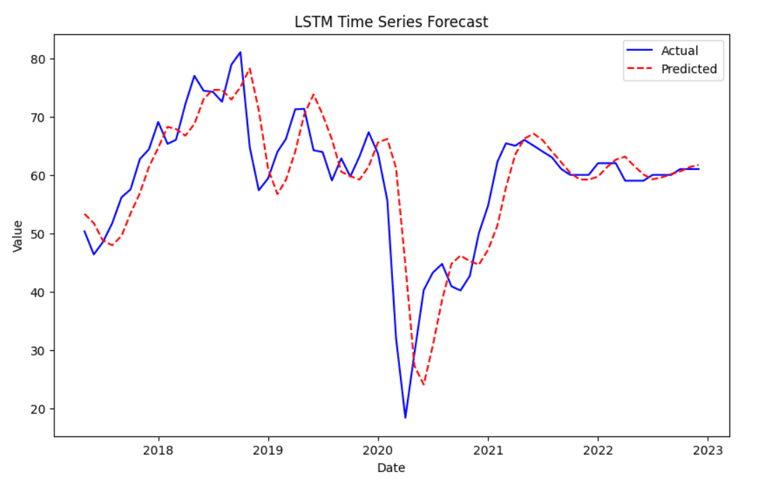
Lastly, we will visualize the anticipated values towards the precise values. The precise values are proven in blue, whereas the anticipated values are in purple with a dashed line.
|
# Plot the precise vs predicted values plt.determine(figsize=(10,6)) plt.plot(df.index[–len(y_test_rescaled):], y_test_rescaled, label=‘Precise’, shade=‘blue’) plt.plot(df.index[–len(y_test_rescaled):], y_pred_rescaled, label=‘Predicted’, shade=‘purple’, linestyle=‘dashed’) plt.title(‘LSTM Time Collection Forecast’) plt.xlabel(‘Date’) plt.ylabel(‘Worth’) plt.legend() plt.present() |
Wrapping Up
On this article, we explored time collection forecasting utilizing completely different strategies.
We began with the ARIMA mannequin. First, we checked if the information was stationary, after which we fitted the mannequin.
Subsequent, we used Exponential Smoothing to seek out developments and seasonality within the knowledge. This helps us see patterns and make higher forecasts.
Lastly, we constructed a Lengthy Brief-Time period Reminiscence mannequin. This mannequin can be taught difficult patterns within the knowledge. We scaled the information, created sequences, and skilled the LSTM to make predictions.
Hopefully this information has been of use to you in protecting these time collection forecasting strategies.
Source link